SVM is a supervised machine learning algorithm which can be used for regression and classification. But it is widely used in classification problems. The main objective of this algorithm is to find a hyperplane in an N-dimensional space(where n is the number of features) that clearly classifies data points. Here a labeled training data is given, this algorithm produces result an optimal hyperplane which categorizes data points. In this context hyperplane is a line that divide a plane in two parts.

How we identify the right hyperplane??

Identify the right hyper-plane (Scenario-1): Here, we have three hyper-planes (A, B and C). Now, identify the right hyper-plane to classify star and circle.

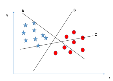
You need to remember a thumb rule to identify the right hyper-plane: “Select the hyper-plane which segregates the two classes better”. In this scenario, hyper-plane “B” has excellently performed this job.

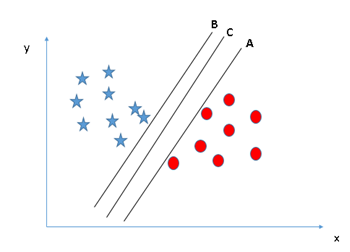
Identify the right hyper-plane (Scenario-2): Here, we have three hyper-planes (A, B and C) and all are segregating the classes well. Now, How can we identify the right hyper-plane?

Here, maximizing the distances between nearest data point (either class) and hyper-plane will help us to decide the right hyper-plane. This distance is called as Margin. Let’s look at the below snapshot:

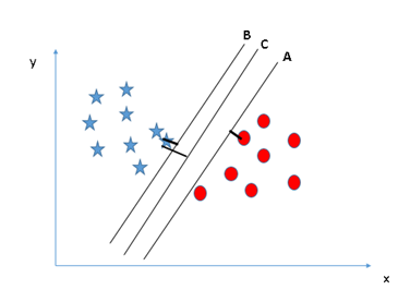
Above, you can see that the margin for hyper-plane C is high as compared to both A and B. Hence, we name the right hyper-plane as C. Another lightning reason for selecting the hyper-plane with higher margin is robustness. If we select a hyper-plane having low margin then there is high chance of miss-classification.

Identify the right hyper-plane (Scenario-3):Hint: Use the rules as discussed in previous section to identify the right hyper-plane

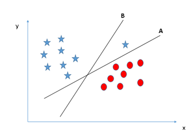
Some of you may have selected the hyper-plane B as it has higher margin compared to A. But, here is the catch, SVM selects the hyper-plane which classifies the classes accurately prior to maximizing margin. Here, hyper-plane B has a classification error and A has classified all correctly. Therefore, the right hyper-plane is A.

Making a little bit complex

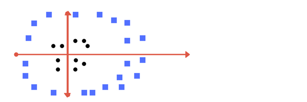
So far so good. Now consider what if we had data as shown in image below? Clearly, there is no line that can separate the two classes in this x-y plane. So what do we do? We apply transformation and add one more dimension as we call it z-axis. Lets assume value of points on z plane, w = x² + y². In this case we can manipulate it as distance of point from z-origin. Now if we plot in z-axis, a clear separation is visible and a line can be drawn .

plot of zy axis. A separation can be made here.

When we transform back this line to original plane, it maps to circular boundary as shown in image E. These transformations are called kernels.

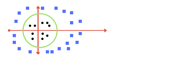
Transforming back to x-y plane, a line transforms to circle.

Let’s see an example:

Iris Flower dataset classification using Support Vector Machine(SVM)

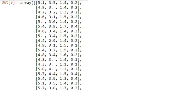
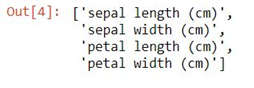
Here we have taken iris flower dataset and by taking four features(sepal length, sepal width, petal length, petal width) we classify the flower is setosa or versicolor or virginica.

#import libraries
import pandas as pd
import matplotlib.pyplot as plt
from sklearn.datasets import load_iris
iris=load_iris()
dir(iris)

Output: ['DESCR', 'data', 'feature_names', 'filename', 'target', 'target_names']

iris.data

iris.feature_names

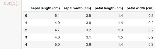
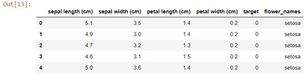
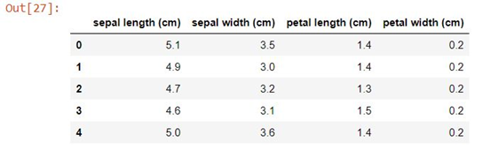
#Create a dataframe by taking values of feature_names

df=pd.DataFrame(iris.data,columns=iris.feature_names)

df.head()

df.shape

Output: (150, 4)

iris.target

df['target']=iris.target

df.head()

iris.target_names

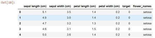
df[df.target==0].head()

df['flower_names']=df.target.apply(lambda x:iris.target_names[x])

df.head()

df0=df[df.target==0]

df1=df[df.target==1]

df2=df[df.target==2]

df0.head()

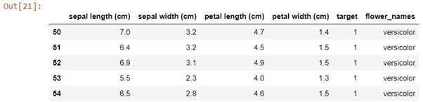
df1.head()

df2.head()

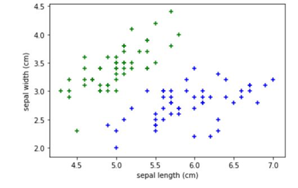
plt.xlabel('sepal length (cm)')
plt.ylabel('sepal width (cm)')
plt.scatter(df0['sepal length (cm)'],df0['sepal width (cm)'],color='green',marker='+')
plt.scatter(df1['sepal length (cm)'],df1['sepal width (cm)'],color='blue',marker='+')
plt.show()

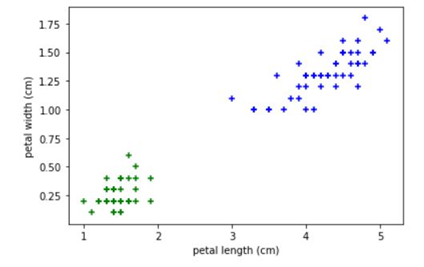
plt.xlabel('petal length (cm)')
plt.ylabel('petal width (cm)')
plt.scatter(df0['petal length (cm)'],df0['petal width (cm)'],color='green',marker='+')
plt.scatter(df1['petal length (cm)'],df1['petal width (cm)'],color='blue',marker='+')
plt.show()

from sklearn.model_selection import train_test_split
X=df.drop(['target','flower_names'],axis='columns')
X.head()

y=df.target
X_train,X_test,y_train,y_test=train_test_split(X,y,test_size=0.2)
len(X_train)
Output: 120

len(X_test)
Output: 30

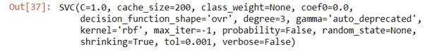
#Create the model
from sklearn.svm import SVC
model=SVC()
model.fit(X_train,y_train)

y_pred=model.predict(X_test)
y_pred

from sklearn.metrics import accuracy_score
print(accuracy_score(y_test,y_pred))
Output: 0.9666666666666667

model.score(X_test,y_test)
Output: 0.9666666666666667